Two-sex time-invariant kinship model specified by age
Source:vignettes/1_3_TwoSex_TimeInvariant_Age.Rmd
1_3_TwoSex_TimeInvariant_Age.RmdLearning Objectives: In this vignette, you will learn how to extend the one-sex kinship model to incorporate both male and female demographic rates. You will understand the implementation of two-sex matrix models, explore how sex-specific mortality and fertility patterns affect kinship structures, and analyze differences in kin availability by sex.
Introduction
Demographic processes fundamental to kinship formation vary significantly between males and females. While one-sex models offer valuable insights into family structures, they overlook these sex differences, which can lead to incomplete understanding of kinship dynamics. Two-sex kinship models address this limitation by incorporating sex-specific demographic rates and tracing both male and female lineages.
Key advantages of two-sex models include:
- Accounting for sex differences in mortality
- Incorporating sex-specific fertility patterns
- Enabling analysis of kin availability by sex
- Allowing for the exploration of sex ratios within kinship networks
- Providing more realistic estimates of kin availability across the life course
In this vignette, we will implement a two-sex time-invariant
kinship model, outlined in Caswell (2022), using the DemoKin package
to understand how sex-specific demographic patterns shape family
structures.
Package Installation
If you haven’t already installed the required packages from the previous vignettes, here’s what you’ll need:
# Install basic data analysis packages
install.packages("dplyr")     # Data manipulation
install.packages("tidyr")     # Data tidying
install.packages("ggplot2")   # Data visualization
install.packages("knitr")     # Document generation

# Install DemoKin
# DemoKin is available on CRAN (https://cran.r-project.org/web/packages/DemoKin/index.html),
# but we'll use the development version on GitHub (https://github.com/IvanWilli/DemoKin):
install.packages("remotes")
remotes::install_github("IvanWilli/DemoKin")
library(DemoKin) # For kinship analysisTwo-Sex Kinship Modeling
Understanding Sex Differences in Demographic Rates
The first step in implementing a two-sex kinship model is to understand the sex differences in demographic rates. Human males and females exhibit distinct mortality and fertility patterns:
- Mortality differences: Males generally experience higher mortality rates at all ages, resulting in shorter life expectancy
- Fertility differences: Males often begin reproduction later and can continue reproducing at older ages
These differences affect kinship structures in several important ways:
- The availability of male versus female relatives (especially at older ages)
- The timing of kin loss experiences (e.g., when fathers versus mothers die)
- The number of descendants for male versus female individuals
For our example, we’ll use data from France (2012), which is included
in the DemoKin package. Let’s examine the sex-specific
mortality and fertility rates:
# Extract sex-specific rates
fra_fert_f <- fra_asfr_sex[,"ff"]    # Female fertility rates
fra_fert_m <- fra_asfr_sex[,"fm"]    # Male fertility rates
fra_surv_f <- fra_surv_sex[,"pf"]    # Female survival probabilities
fra_surv_m <- fra_surv_sex[,"pm"]    # Male survival probabilities

# Compare total fertility rates by sex
cat("Difference in TFR (male - female):", sum(fra_fert_m) - sum(fra_fert_f))
## Difference in TFR (male - female): -0.0115
# Visualize sex differences in demographic rates
data.frame(value = c(fra_fert_f, fra_fert_m, fra_surv_f, fra_surv_m),
           age = rep(0:100, 4),
           sex = rep(c(rep("f", 101), rep("m", 101)), 2),
           risk = c(rep("fertility rate", 101 * 2), rep("survival probability", 101 * 2))) %>%
  ggplot(aes(age, value, col=sex)) +
  geom_line(linewidth = 1) +
  labs(
    title = "Sex-specific demographic rates in France (2012)",
    x = "Age",
    y = "Rate",
    color = "Sex"
  ) +
  facet_wrap(~ risk, scales = "free_y") +
  theme_bw()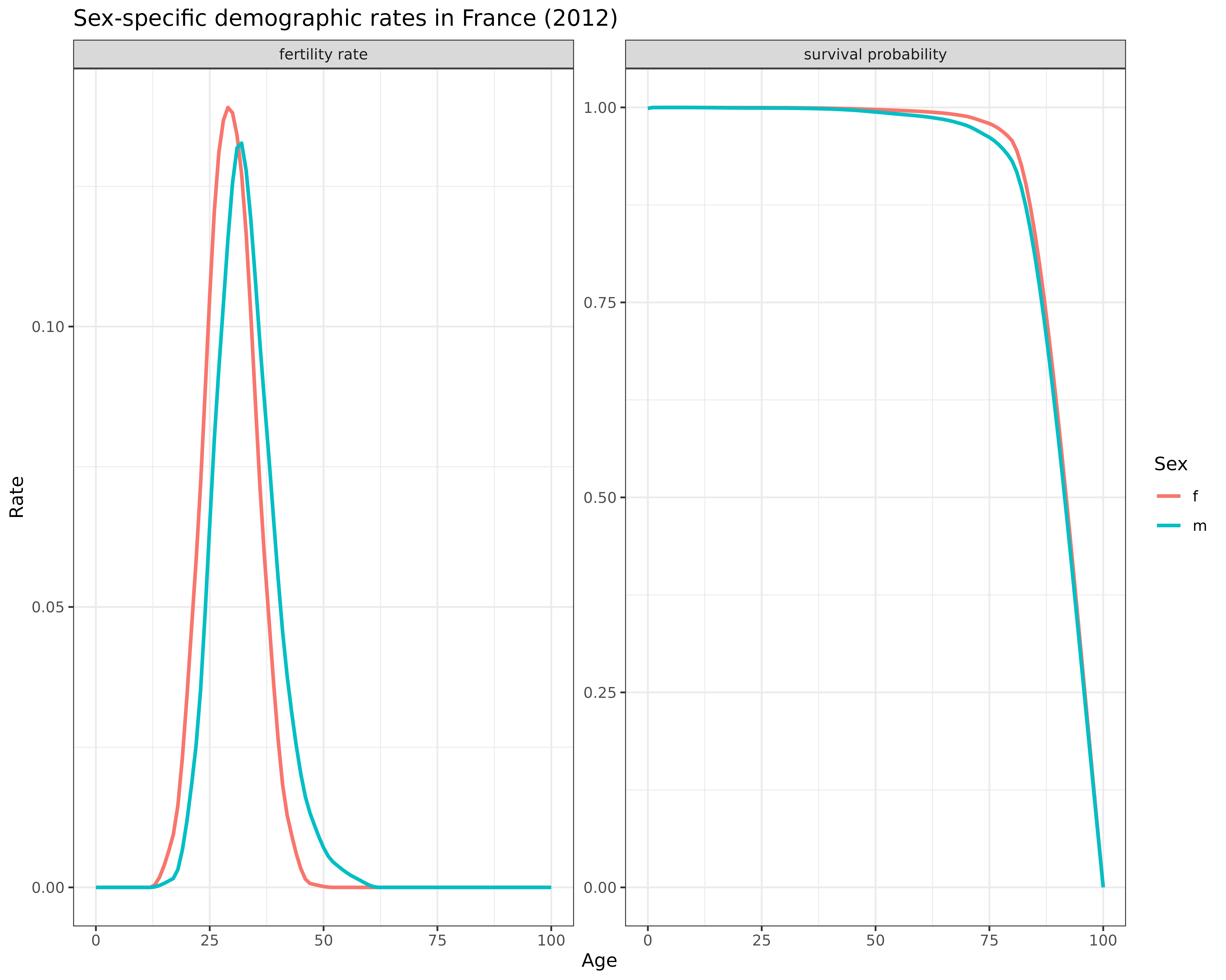
Interpretation: The graphs reveal important sex differences in demographic rates:
Fertility patterns: While total fertility rates are nearly identical between males and females (difference of only 0.01), the age patterns differ substantially. Male fertility occurs at later ages and has a wider distribution, reflecting the tendency for men to father children at older ages compared to women.
Survival probabilities: Females have higher survival probabilities at most of adult and old ages. This pattern leads to sex imbalances in older populations and affects the availability of different types of relatives.
These sex differences in demographic rates will shape kinship networks in ways that one-sex models cannot capture.
Implementing the Two-Sex Model
We now introduce the function kin2sex, which extends the
one-sex function kin to incorporate sex-specific rates. The
key differences are:
- We need to provide both female and male demographic rates
- We must specify the sex of the focal individual
- We need to indicate the sex ratio at birth (proportion of births that are female)
Let’s implement a two-sex time-varying model for France:
kin_result <- kin2sex(
  pf = fra_surv_f,        # Female survival probabilities
  pm = fra_surv_m,        # Male survival probabilities
  ff = fra_fert_f,        # Female fertility rates
  fm = fra_fert_m,        # Male fertility rates
  time_invariant = TRUE,  # Use time-invariant model
  sex_focal = "f",        # Focus on female focal individuals
  birth_female = .5       # Proportion of births that are female
)
The output of kin2sex is similar to that of
kin, with an additional column sex_kin that
specifies the sex of each relative.
Living Relatives by Sex
Let’s examine how the number of living relatives differs by sex across the life course of a female focal individual:
# Group specific kin types and filter for key relationships
kin_out <- kin_result$kin_summary %>%
  mutate(kin = case_when(kin %in% c("ys", "os") ~ "s",      # Siblings
                         kin %in% c("ya", "oa") ~ "a",    # Aunts/uncles
                         TRUE ~ kin)) %>%
  filter(kin %in% c("d", "m", "gm", "ggm", "s", "a"))     # Select key relationships

# Visualize living kin by sex
kin_out %>%
  group_by(kin, age_focal, sex_kin) %>%
  summarise(count = sum(count_living)) %>%
  ggplot(aes(age_focal, count, fill = sex_kin)) +
  geom_area() +
  labs(
    title = "Expected number of living relatives by sex",
    subtitle = "Female focal individual, France 2012",
    x = "Age of focal individual",
    y = "Number of living relatives",
    fill = "Sex of relative"
  ) +
  theme_bw() +
  facet_wrap(~kin, labeller = labeller(
    kin = c("a" = "Aunts/Uncles", "d" = "Children",
            "gm" = "Grandparents", "ggm" = "Great-grandparents",
            "m" = "Parents", "s" = "Siblings")
  ))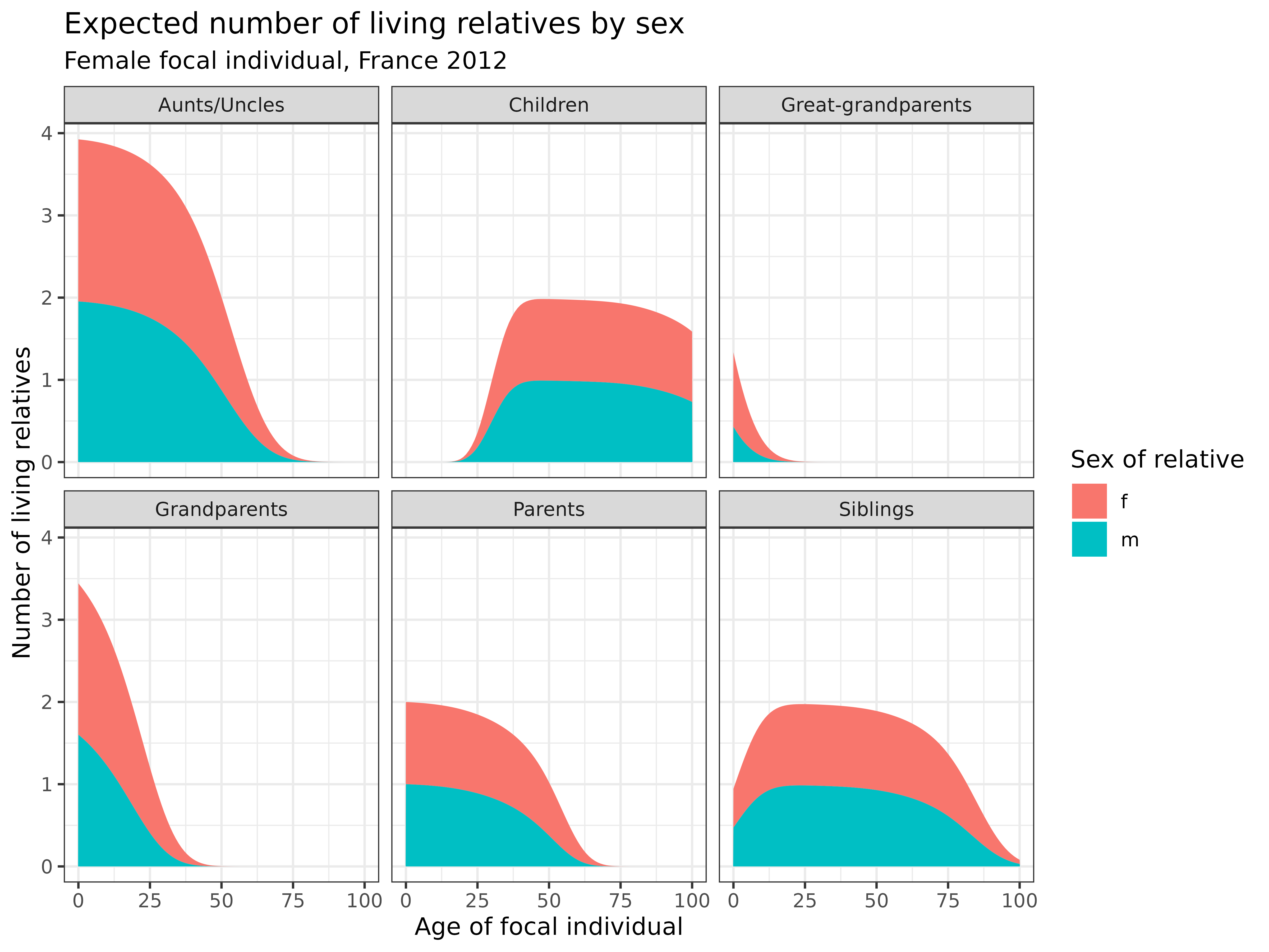
Interpretation: These stacked area plots reveal how the sex composition of living relatives changes across the life course:
- Parents (m): Fathers (blue) die earlier than mothers (red), leading to a predominance of mothers at older ages
- Grandparents (gm): Even at birth, grandmothers outnumber grandfathers due to mortality in the grandparental generation
- Great-grandparents (ggm): Shows an even stronger female predominance due to compounded mortality differences across generations
- Siblings (s): Brothers die earlier than sisters, leading to a higher proportion of sisters at older ages
- Children (d): Starts with an even sex ratio, with slight female predominance at older ages due to higher male mortality
These patterns highlight the importance of accounting for sex differences in kinship models, especially when studying older populations.
Understanding Kinship Terminology in Two-Sex Models
When using the kin2sex function, it’s important to
understand how relationship codes work:
# Example of how to identify specific relatives by sex
kin_result$kin_summary %>%
  filter(kin == "d", sex_kin == "m") %>%  # This selects sons (male children)
  head()
## # A tibble: 6 × 11
## age_focal kin sex_kin year cohort count_living mean_age sd_age count_dead
## <int> <chr> <chr> <lgl> <lgl> <dbl> <dbl> <dbl> <dbl>
## 1 0 d m NA NA 0 NaN NaN 0
## 2 1 d m NA NA 0 NaN NaN 0
## 3 2 d m NA NA 0 NaN NaN 0
## 4 3 d m NA NA 0 NaN NaN 0
## 5 4 d m NA NA 0 NaN NaN 0
## 6 5 d m NA NA 0 NaN NaN 0
## # ℹ 2 more variables: count_cum_dead <dbl>, mean_age_lost <dbl>The function uses the same relationship codes as the one-sex model
(see demokin_codes()), but now each relative has a
specified sex. For example:
-
kin = "d", sex_kin = "f"refers to daughters -
kin = "d", sex_kin = "m"refers to sons -
kin = "m", sex_kin = "f"refers to mothers -
kin = "m", sex_kin = "m"refers to fathers
This coding system allows for flexible analysis of specific relative types while maintaining compatibility with the one-sex model.
Sex Ratios in Kinship Networks
Sex ratios (males per female) are a traditional measure in demography that can provide insights into kinship structures. Let’s examine how sex ratios vary across different types of relatives:
# Calculate sex ratios (males per female) by kin type and age
kin_out %>%
  group_by(kin, age_focal) %>%
  summarise(sex_ratio = sum(count_living[sex_kin == "m"], na.rm = TRUE) /
                        sum(count_living[sex_kin == "f"], na.rm = TRUE)) %>%
  ggplot(aes(age_focal, sex_ratio)) +
  geom_line(linewidth = 1) +
  geom_hline(yintercept = 1, linetype = "dashed", color = "gray50") +
  labs(
    title = "Sex ratios of living relatives across the life course",
    subtitle = "Males per female, France 2012",
    x = "Age of focal individual",
    y = "Sex ratio (m/f)"
  ) +
  theme_bw() +
  facet_wrap(~kin, scales = "free", labeller = labeller(
    kin = c("a" = "Aunts/Uncles", "d" = "Children",
            "gm" = "Grandparents", "ggm" = "Great-grandparents",
            "m" = "Parents", "s" = "Siblings")
  ))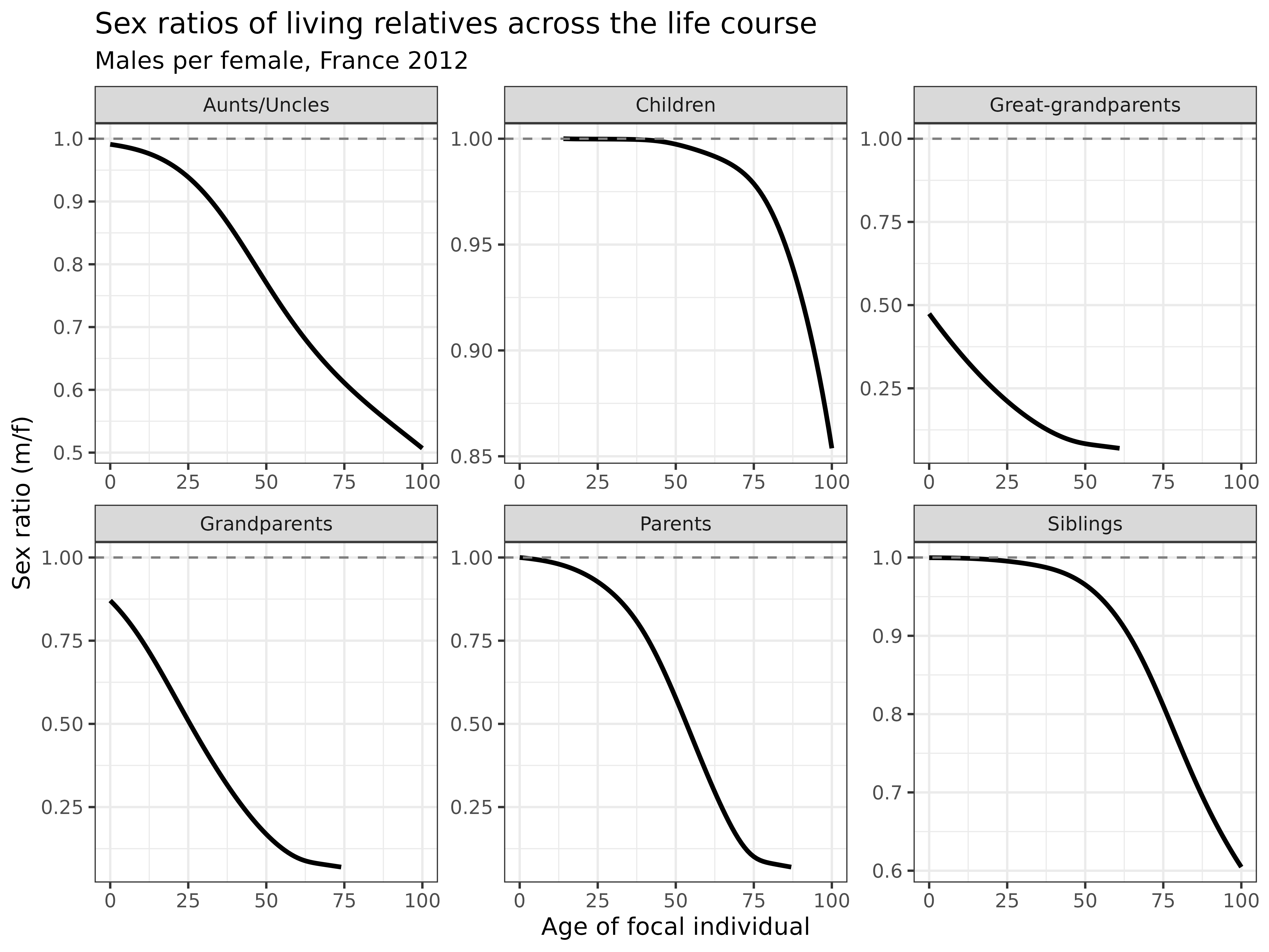
Interpretation: The sex ratio plots reveal several important patterns:
- Parents: The sex ratio starts at 1 (equal numbers of mothers and fathers) but declines rapidly with age, reflecting higher male mortality
- Grandparents: Even at birth, the sex ratio is below 1, with a 25-year-old having only about 0.5 grandfathers per grandmother
- Great-grandparents: Shows even more extreme female predominance
- Children: Maintains a sex ratio close to 1 throughout life, with slight declines at older ages
- Siblings: Shows gradual decline in sex ratio with age due to higher male mortality
These sex ratios have important implications for care relationships and support networks, particularly in older populations where female relatives predominate.
Timing of Kin Loss by Sex
The experience of losing relatives differs by the sex of those relatives. Let’s examine how the timing of kin loss varies by sex:
# Visualize dead kin by sex
kin_out %>%
  group_by(kin, sex_kin, age_focal) %>%
  summarise(count = sum(count_dead)) %>%
  ggplot(aes(age_focal, count, color = sex_kin)) +
  geom_line(linewidth = 1) +
  labs(
    title = "Number of deceased relatives by sex",
    subtitle = "Female focal individual, France 2012",
    x = "Age of focal individual",
    y = "Number of deceased relatives",
    color = "Sex of relative"
  ) +
  theme_bw() +
  facet_wrap(~kin, scales = "free", labeller = labeller(
    kin = c("a" = "Aunts/Uncles", "d" = "Children",
            "gm" = "Grandparents", "ggm" = "Great-grandparents",
            "m" = "Parents", "s" = "Siblings")
  ))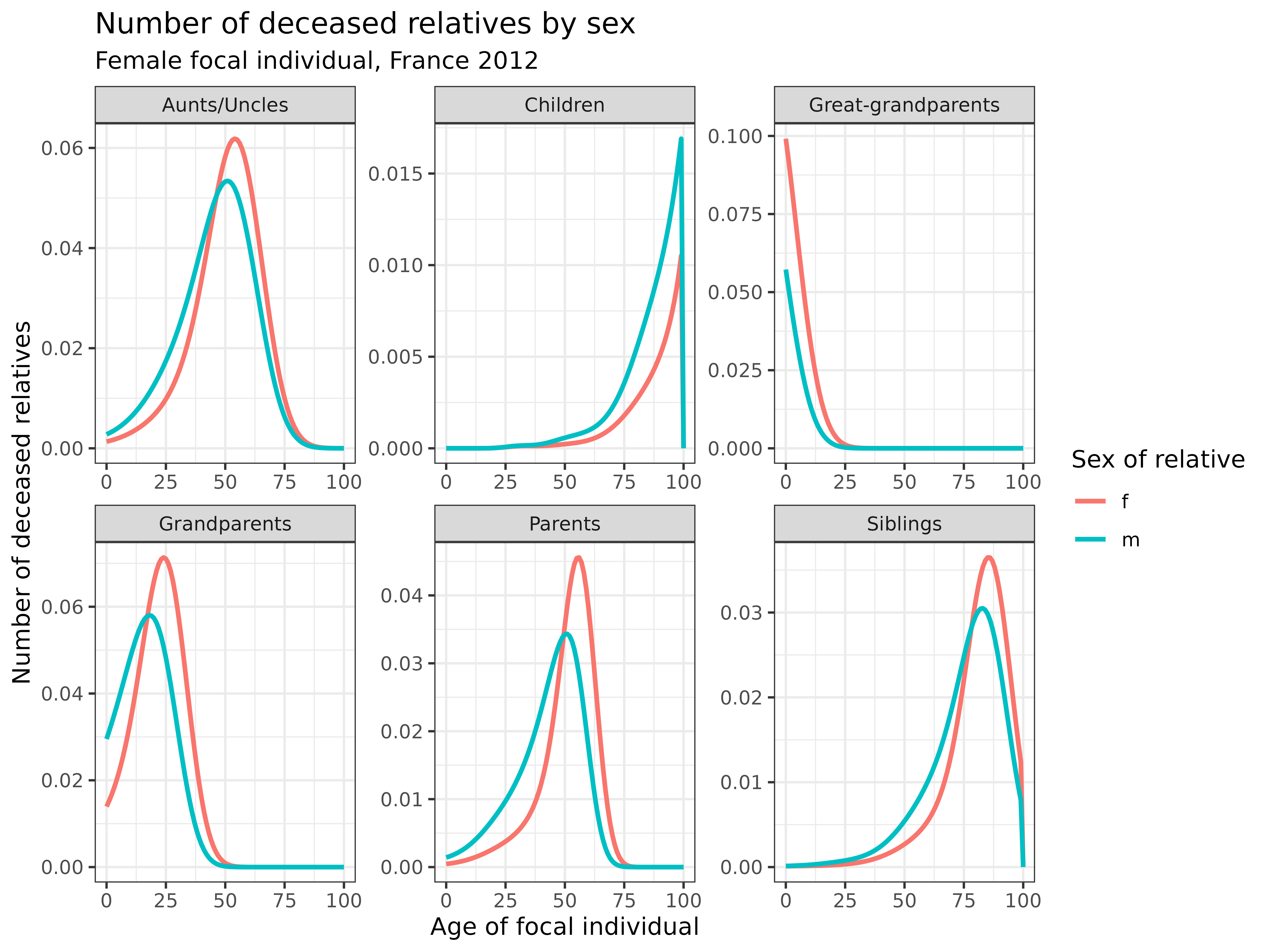
Interpretation: These curves show how the experience of losing relatives differs by sex:
- Parents: The loss of fathers (blue) occurs earlier than the loss of mothers (red)
- Grandparents: Grandfather are often lost before birth or early in life, while grandmothers tend to be lost later
- Siblings: Brothers are lost at higher rates than sisters before old ages (75+)
- Children: While rare, the loss of sons occurs at higher rates than daughters
Understanding these patterns is important for studying bereavement experiences and their impacts across the life course.
Applications of Two-Sex Kinship Models
Two-sex kinship models have numerous applications in demographic and social research:
Gender and care: Women typically provide more informal care to relatives than men. Two-sex models can help quantify potential care burdens by examining the availability of different types of relatives by sex.
Kinship networks in aging societies: As populations age, the sex composition of available kin changes dramatically. Two-sex models allow us to project these changes and their implications for social support.
Intergenerational transfers: Resources often flow differently between male and female relatives. Two-sex models provide the demographic foundation for studying these gendered patterns.
Demographic transitions: Sex differences in mortality and fertility change during demographic transitions, reshaping kinship networks in ways that one-sex models cannot capture.
Demographic shocks: Events like wars often affect males and females differently, with long-lasting impacts on kinship structures. Two-sex models can capture these effects.
Conclusion
In this vignette, we’ve explored how to implement two-sex kinship
models using the DemoKin package. By incorporating
sex-specific mortality and fertility rates, these models reveal
important patterns that one-sex models cannot capture:
- Female predominance among older relatives due to sex differences in mortality
- Systematic differences in the timing of kin loss by sex, with male kin typically lost earlier
- Varying sex ratios within kinship networks by relationship type and age
- Distinct age distributions of relatives by sex
These insights have significant implications for understanding care relationships, intergenerational transfers, and support systems in aging societies. The two-sex approach substantially enhances our understanding of how gender shapes family structures across the life course, providing a more realistic foundation for both research and policy development.