Two-sex time-varying kinship model specified by age and stage
Source:vignettes/2_2_TwoSex_TimeVarying_AgeStage.Rmd
2_2_TwoSex_TimeVarying_AgeStage.RmdLearning Objectives: In this vignette, you will learn how to implement a kinship model that combines both two-sex and time-varying approaches with multiple stages. You will understand how to incorporate sex-specific demographic rates that change over time, analyze the effects of demographic transitions on kinship structures by sex and stage, and explore applications with different stage variables such as parity and education.
Introduction
In this final vignette, we integrate all elements from previous tutorials into the most comprehensive kinship model available: a two-sex time-varying multi-state model. This framework simultaneously accounts for:
- Sex differences in demographic rates
- Historical changes over time
- Stage-based transitions (like parity or education)
- Joint distributions of age, sex, and stage among relatives
Building on previous Caswell and colleagues’ theoretical developments
(2019, 2020, 2022; 2021), Butterick and
others (2025) created an integral approach
providing unprecedented analytical power for understanding complex
family structures. We’ll apply this comprehensive model using the
kin_multi_stage_time_variant_2sex function, exploring two
examples: one using parity and another using educational attainment to
demonstrate how these models illuminate contemporary family dynamics in
ways simpler models cannot.
Package Installation
If you haven’t already installed the required packages from the previous vignettes, here’s what you’ll need:
# Install basic data analysis packages
install.packages("dplyr")     # Data manipulation
install.packages("tidyr")     # Data tidying
install.packages("ggplot2")   # Data visualization
install.packages("knitr")     # Document generation
install.packages("Matrix")    # Matrix operations

# Install DemoKin
# DemoKin is available on CRAN (https://cran.r-project.org/web/packages/DemoKin/index.html),
# but we'll use the development version on GitHub (https://github.com/IvanWilli/DemoKin):
install.packages("remotes")
remotes::install_github("IvanWilli/DemoKin")
library(DemoKin)Two-Sex Time-Varying Multi-State Models
The kin_multi_stage_time_variant_2sex function in the
DemoKin package allows us to implement a comprehensive
kinship model that accounts for sex, time, and stage simultaneously.
This function computes stage-specific kinship networks across both sexes
for an average member of a population (focal) under time-varying
demographic rates.
The model estimates:
- The number of relatives of each type
- The age distribution of relatives
- The sex distribution of relatives
- The stage distribution of relatives
- How these distributions change over the life course of Focal
- How they vary by Focal’s birth cohort
Model Components and Requirements
The two-sex time-varying multi-state model requires several inputs:
- Sex-specific mortality rates by stage over time: How survival probabilities differ between males and females of different stages across historical periods
- Sex-specific fertility rates by stage over time: How fertility patterns differ between males and females of different stages across historical periods
- Sex-specific transition rates between stages over time: How individuals move between stages at each age, potentially differing by sex
- Sex ratio at birth: The proportion of births that are female
- Birth redistribution matrices: How newborns are distributed across stages
- Sex and initial stage of the focal individual: The characteristics of the person whose kin network we’re analyzing
In the following sections, we’ll explore two examples of this model using different stage variables: parity and education.
Example 1: Parity as the Stage Variable
Data Preparation
In our first example, we’ll use parity (number of children already born) as our stage variable. We’ll use data from the United Kingdom ranging from 1965 to 2022, sourced from the Human Mortality Database and the Office for National Statistics.
Due to data limitations, we make some simplifying assumptions:
- Fertility rates vary with time and parity but are the same across sexes (the “androgynous approximation”)
- Mortality rates vary with time and sex but are the same across parity classes
- Parity progression probabilities vary with time but are the same across sexes
Let’s load the pre-processed UK data:
# Load pre-processed data for UK
F_mat_fem <- Female_parity_fert_list_UK       # Female fertility by parity
F_mat_male <- Female_parity_fert_list_UK      # Male fertility (same as female due to androgynous approximation)
T_mat_fem <- Parity_transfers_by_age_list_UK  # Female parity transitions
T_mat_male <- Parity_transfers_by_age_list_UK # Male parity transitions (same as female)
U_mat_fem <- Female_parity_mortality_list_UK  # Female survival
U_mat_male <- Male_parity_mortality_list_UK   # Male survival
These lists contain period-specific demographic rates:
-
U_mat_fem/U_mat_male: Lists of matrices containing survival probabilities by age (rows) and parity (columns) from 1965-2022 -
F_mat_fem/F_mat_male: Lists of matrices containing fertility rates by age and parity -
T_mat_fem/T_mat_male: Lists of transition matrices showing probabilities of moving between parity states
Careful: Actual application assumes that always newborn will be assign to age 0.
Running the Parity Model
Now let’s implement the two-sex time-varying multi-state model with parity as the stage variable:
Note: This model run takes approximately 30 minutes to complete, so we let to the reader its run.
# Define time period and parameters
no_years <- 40  # Run the model for 40 years (1965-2005)

# Run the model
kin_out_1965_2005 <-
  kin_multi_stage_time_variant_2sex(
    U_list_females = U_mat_fem[1:(1+no_years)],        # Female survival matrices
    U_list_males = U_mat_male[1:(1+no_years)],         # Male survival matrices
    F_list_females = F_mat_fem[1:(1+no_years)],        # Female fertility matrices
    F_list_males = F_mat_male[1:(1+no_years)],         # Male fertility matrices
    T_list_females = T_mat_fem[1:(1+no_years)],        # Female transition matrices
    T_list_males = T_mat_fem[1:(1+no_years)],          # Male transition matrices
    birth_female = 1 - 0.51,                           # UK sex ratio (49% female)
    parity = TRUE,                                      # Stages represent parity
    output_kin = c("d", "oa", "ys", "os"),             # Selected kin types
    summary_kin = TRUE,                                 # Produce summary statistics
    sex_Focal = "Female",                               # Focal is female
    initial_stage_Focal = 1,                            # Focal starts at parity 0
    output_years = c(1965, 1975, 1985, 1995, 2005)     # Selected output years
  )
Now we need to recode the stage variables to show meaningful parity labels:
# After running the model, recode the parity stage values
kin_out_1965_2005$kin_summary <-
  kin_out_1965_2005$kin_summary %>%
  mutate(stage_kin = factor(as.numeric(stage_kin) - 1,
                           levels = c(0, 1, 2, 3, 4, 5),
                           labels = c("0", "1", "2", "3", "4", "5+")))

# Do the same for the kin_full dataframe if you're using it
kin_out_1965_2005$kin_full <-
  kin_out_1965_2005$kin_full %>%
  mutate(stage_kin = factor(as.numeric(stage_kin) - 1,
                           levels = c(0, 1, 2, 3, 4, 5),
                           labels = c("0", "1", "2", "3", "4", "5+")))
Analyzing Kin Counts by Parity
Let’s examine the structure of the output:
head(kin_out_1965_2005$kin_summary)The output includes:
-
age_focal: Age of the focal individual -
kin_stage: Stage (parity) of the relatives -
sex_kin: Sex of the relatives -
year: Calendar year of observation -
kin: Type of relative (d = children, oa = older aunts/uncles, etc.) -
living: Expected number of living relatives -
cohort: Birth cohort of the focal individual
Period Analysis of Kin by Parity
Let’s visualize the distribution of older aunts and uncles by parity for different ages of Focal across different calendar years.
We first restrict Focal’s kinship network to aunts and uncles older
than Focal’s mother by setting kin == “oa”. We visualize
the marginal parity distributions of kin: stage_kin, for
each age of Focal age_focal, using different color schemes.
Implicit in the below plot is that we really plot Focal’s born into
different cohort – i.e., in the 2005 panel we show a 50
year old Focal was born in 1955, while a 40 year old Focal was born in
1965.
kin_out_1965_2005$kin_summary %>%
  filter(kin == "oa") %>%
  ggplot(aes(x = age_focal, y = living, color = stage_kin, fill = stage_kin)) +
  geom_bar(position = "stack", stat = "identity") +
  facet_grid(sex_kin ~ year) +
  scale_x_continuous(breaks = c(0,10,20,30,40,50,60,70,80,90,100)) +
  theme_bw() +
  theme(axis.text.x = element_text(angle = 90, vjust = 0.5)) +
  labs(
    title = "Parity distribution of older aunts and uncles by Focal's age",
    subtitle = "United Kingdom, 1965-2005",
    x = "Age of focal individual",
    y = "Number of older aunts and uncles",
    fill = "Parity",
    color = "Parity"
  )
We could also consider any other kin in Focal’s network, for
instance, offspring using kin == “d”:
kin_out_1965_2005$kin_summary %>%
  filter(kin == "d") %>%
  ggplot(aes(x = age_focal, y = living, color = stage_kin, fill = stage_kin)) +
  geom_bar(position = "stack", stat = "identity") +
  facet_grid(sex_kin ~ year) +
  scale_x_continuous(breaks = c(0,10,20,30,40,50,60,70,80,90,100)) +
  theme_bw() +
  theme(axis.text.x = element_text(angle = 90, vjust = 0.5)) +
  labs(
    title = "Parity distribution of children by Focal's age",
    subtitle = "United Kingdom, 1965-2005",
    x = "Age of focal individual",
    y = "Number of children",
    fill = "Parity",
    color = "Parity"
  )
Cohort Analysis of Kin by Parity
Since we only ran the model for 40 years (between 1965-2005), there is very little scope to view kinship as cohort-specific.
We can however compare cohorts for 40-year segments of Focal’s life.
Below, following from the above example, we once again consider
offspring and only show Focals born of cohort 1910, 1925,
or 1965:
kin_out_1965_2005$kin_summary %>%
  filter(kin == "d", cohort %in% c(1910, 1925, 1965)) %>%
  ggplot(aes(x = age_focal, y = living, color = stage_kin, fill = stage_kin)) +
  geom_bar(position = "stack", stat = "identity") +
  facet_grid(sex_kin ~ cohort) +
  theme_bw() +
  theme(axis.text.x = element_text(angle = 90, vjust = 0.5)) +
  labs(
    title = "Parity distribution of offspring by birth cohort",
    subtitle = "United Kingdom, ages observed between 1965-2005",
    x = "Age of focal individual",
    y = "Number of offspring",
    fill = "Parity",
    color = "Parity"
)Interpretation:
- The 1910 cohort (observed at ages 55-95): Most offspring have already completed their childbearing, showing a mix of parity states
- The 1925 cohort (observed at ages 40-80): Offspring are observed during and after their reproductive years
- The 1965 cohort (observed at ages 0-40): Initially, all offspring are in parity 0, gradually transitioning to higher parities as they age
Age Distribution of Kin by Parity
For more detailed analysis, we can examine the age and parity distribution of specific relatives. Let’s look at the younger siblings of a 50-year-old Focal across different years:
kin_out_1965_2005$kin_full %>%
  filter(kin == "ys",
         age_focal == 50) %>%
  ggplot(aes(x = age_kin, y = living, color = stage_kin, fill = stage_kin)) +
  geom_bar(position = "stack", stat = "identity") +
  facet_grid(sex_kin ~ year) +
  scale_x_continuous(breaks = c(0,10,20,30,40,50,60,70,80,90,100)) +
  theme_bw() +
  theme(axis.text.x = element_text(angle = 90, vjust = 0.5)) +
  labs(
    title = "Age and parity distribution of younger siblings",
    subtitle = "For a 50-year-old focal individual, United Kingdom, 1965-2005",
    x = "Age of sibling",
    y = "Number of younger siblings",
    fill = "Parity",
    color = "Parity"
  )
Notice the discontinuity along the x-axis at age 50. This reflects the fact that younger siblings cannot be older than Focal (by definition). Similarly, when we examine older siblings, we’ll see they cannot be younger than Focal.
With a simple manipulation of the output data frame, we can also plot the age and parity distribution of all siblings combined:
kin_out_1965_2005$kin_full %>%
  filter((kin == "ys" | kin == "os"),
         age_focal == 50) %>%
  pivot_wider(names_from = kin, values_from = living) %>%
  mutate(count = `ys` + `os`) %>%
  ggplot(aes(x = age_kin, y = count, color = stage_kin, fill = stage_kin)) +
  geom_bar(position = "stack", stat = "identity") +
  facet_grid(sex_kin ~ year) +
  scale_x_continuous(breaks = c(0,10,20,30,40,50,60,70,80,90,100)) +
  theme_bw() +
  theme(axis.text.x = element_text(angle = 90, vjust = 0.5)) +
  labs(
    title = "Age and parity distribution of all siblings",
    subtitle = "For a 50-year-old focal individual, United Kingdom, 1965-2005",
    x = "Age of sibling",
    y = "Number of siblings",
    fill = "Parity",
    color = "Parity"
  )
Example 2: Education as the Stage Variable
Data Preparation
In our second example, we’ll use educational attainment as our stage variable. The data is for Singapore ranging from 2020 to 2090, sourced from the Wittgenstein Center. The data is aggregated into 5-year age groups and 5-year time intervals.
Some simplifying assumptions we make due to data availability:
- Fertility rates vary with time and education but are identical for both sexes (androgynous approximation)
- Age-specific education transition probabilities vary over time but not by sex
- Educational transitions for young children follow Singapore’s Compulsory Education Act
- Demographic rates before 2020 are assumed stable (time-invariant)
Let’s load the pre-processed Singapore data:
This data includes:
-
U_mat_fem_edu/U_mat_male_edu: Lists of matrices containing survival probabilities by age (rows) and education (columns) from 2020-2090 -
F_mat_fem_edu/F_mat_male_edu: Lists of matrices containing fertility rates by age and education -
T_mat_fem_edu/T_mat_male_edu: Lists of transition matrices showing probabilities of moving between education states -
H_mat_edu: List of matrices that redistribute newborns to age-class 1 and “no education” category
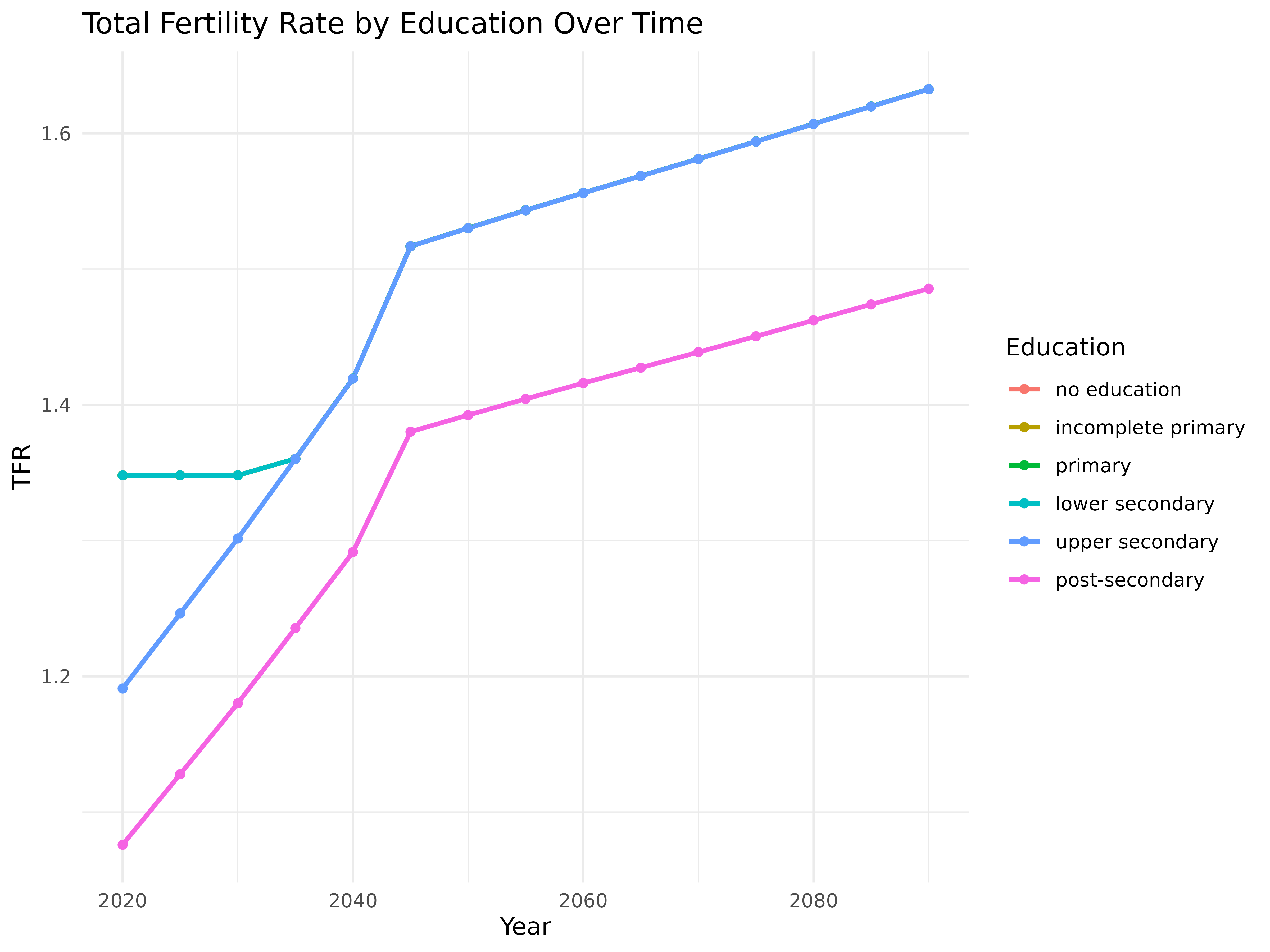
Before running the model, let’s examine some trends in the data:
# Calculate and plot Total Fertility Rate by education level over time
tfr_data <- lapply(seq_along(F_mat_fem_edu), function(i) {
  col_sums <- colSums(F_mat_fem_edu[[i]])
  data.frame(
    year = 2020 + (i - 1) * 5,
    education = factor(colnames(F_mat_fem_edu[[i]]),
                      levels = c("e1", "e2", "e3", "e4", "e5", "e6"),
                      labels = c("no education", "incomplete primary",
                                "primary", "lower secondary",
                                "upper secondary", "post-secondary")),
    tfr = col_sums
  )
})

tfr_df <- do.call(rbind, tfr_data)

# Plot TFR trends
ggplot(tfr_df, aes(x = year, y = tfr, color = education, group = education)) +
  geom_line(size = 1) +
  geom_point() +
  theme_minimal() +
  labs(
    title = "Total Fertility Rate by Education Over Time",
    x = "Year",
    y = "TFR",
    color = "Education"
  )
Running the Education Model
Now let’s implement the two-sex time-varying multi-state model with education as the stage variable:
# Define time period and parameters
time_range <- seq(2020, 2090, 5)
no_years <- length(time_range) - 1
output_year <- seq(1, no_years + 1, 1)

# Run the model
kin_out_2020_2090 <-
  kin_multi_stage_time_variant_2sex(
    U_list_females = U_mat_fem_edu[1:(1+no_years)],     # Female survival matrices
    U_list_males = U_mat_male_edu[1:(1+no_years)],      # Male survival matrices
    F_list_females = F_mat_fem_edu[1:(1+no_years)],     # Female fertility matrices
    F_list_males = F_mat_male_edu[1:(1+no_years)],      # Male fertility matrices
    T_list_females = T_mat_fem_edu[1:(1+no_years)],     # Female transition matrices
    T_list_males = T_mat_fem_edu[1:(1+no_years)],       # Male transition matrices
    birth_female = 1/(1.06+1),                          # Singapore sex ratio (48.5% female)
    parity = FALSE,                                      # Stages represent education
    summary_kin = TRUE,                                  # Produce summary statistics
    sex_Focal = "Female",                                # Focal is female
    initial_stage_Focal = 1,                             # Focal starts with no education
    output_years = output_year                           # All years
  )
Note: This model run takes approximately 3 minutes to complete.
Now we need to recode the stage variables to show meaningful educational labels and convert years/ages to real values (since we used 5-year intervals):
# Recode year and age variables to show correct values
kin_out_2020_2090$kin_summary <-
  kin_out_2020_2090$kin_summary %>%
  mutate(year = (year-1)*5+min(time_range),
         age_focal = age_focal*5,
         cohort = year - age_focal,
         stage_kin = factor(stage_kin, levels = c(1, 2, 3, 4, 5, 6),
                       labels = c(
                         "no education",
                         "incomplete primary",
                         "primary",
                         "lower secondary",
                         "upper secondary",
                         "post-secondary"
                       )))

kin_out_2020_2090$kin_full <-
  kin_out_2020_2090$kin_full %>%
  mutate(year = (year-1)*5+min(time_range),
         age_focal = age_focal*5,
         age_kin = age_kin*5,
         cohort = year - age_focal,
         stage_kin = factor(stage_kin, levels = c(1, 2, 3, 4, 5, 6),
                       labels = c(
                         "no education",
                         "incomplete primary",
                         "primary",
                         "lower secondary",
                         "upper secondary",
                         "post-secondary"
                       )))
Analyzing Kin by Educational Attainment
Cohort Analysis of Kin by Education
First, let’s visualize the total number of living kin by educational attainment for a woman born in 2020 in Singapore:
kin_out_2020_2090$kin_summary %>%
  # Exclude Focal from the analysis
  filter(kin != "Focal") %>%
  filter(cohort == 2020) %>%
  # rename_kin(sex = "2sex") %>%
  summarise(count = sum(living), .by = c(stage_kin, age_focal)) %>%
  ggplot(aes(x = age_focal, y = count, fill = stage_kin)) +
  geom_area(colour = "black") +
  labs(
    title = "Total living kin by educational attainment over the life course",
    subtitle = "For a woman born in 2020, Singapore",
    y = "Expected number of living kin",
    x = "Age of focal individual",
    fill = "Educational attainment"
  ) +
  theme_bw() +
  theme(legend.position = "bottom")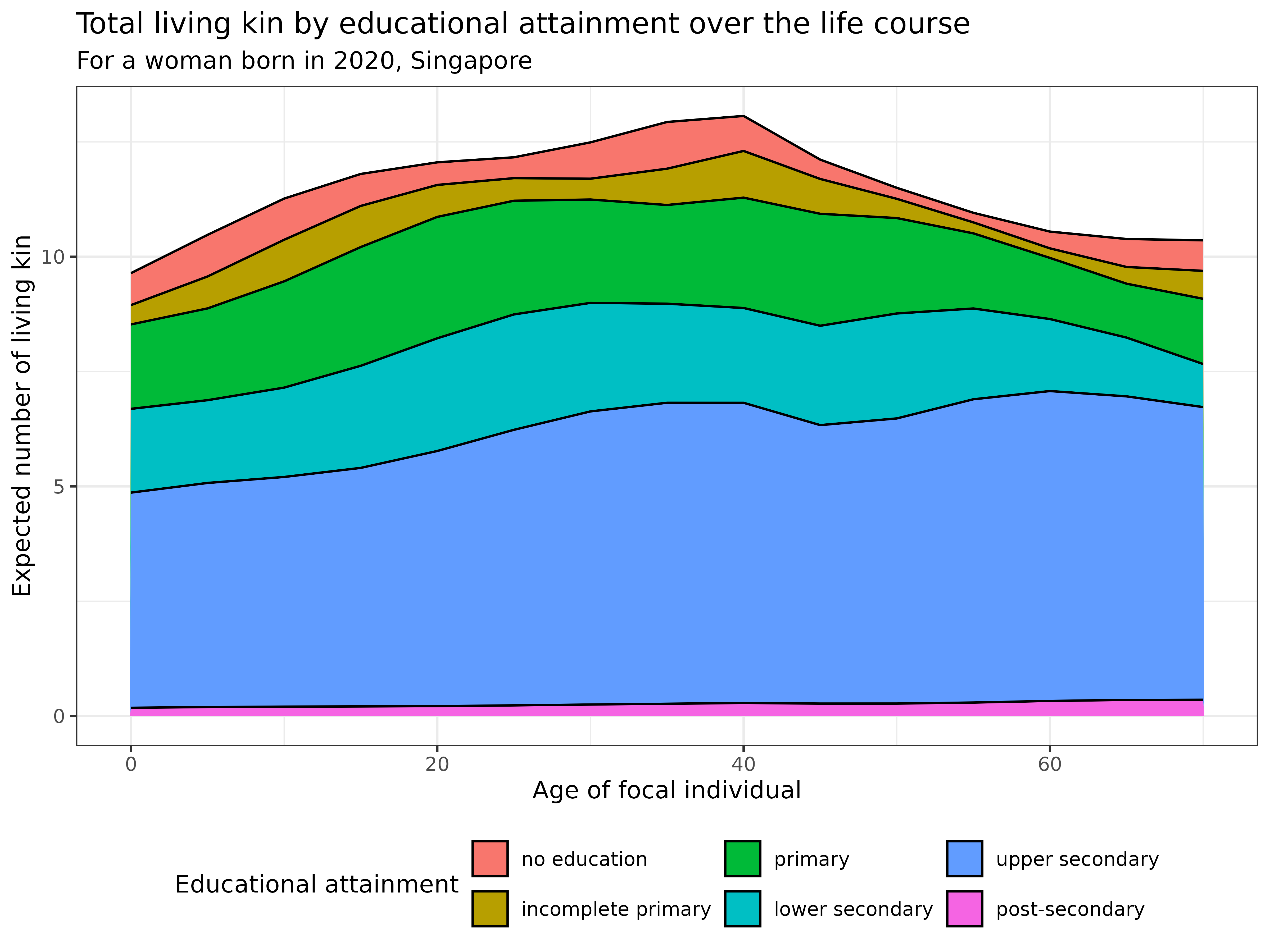
Now let’s look at specific types of relatives:
kin_out_2020_2090$kin_summary %>%
  filter(kin %in% c("d", "gd", "m", "gm")) %>%
  filter(cohort == 2020) %>%
  # rename_kin(sex = "2sex") %>%
  summarise(count = sum(living), .by = c(kin, stage_kin, age_focal)) %>%
  ggplot(aes(x = age_focal, y = count, fill = stage_kin)) +
  geom_area(colour = "black") +
  labs(
    title = "Living kin by educational attainment over the life course",
    subtitle = "For a woman born in 2020, Singapore",
    y = "Expected number of living kin",
    x = "Age of focal individual",
    fill = "Educational attainment"
  ) +
  facet_wrap(. ~ kin) +
  theme_bw() +
  theme(legend.position = "bottom")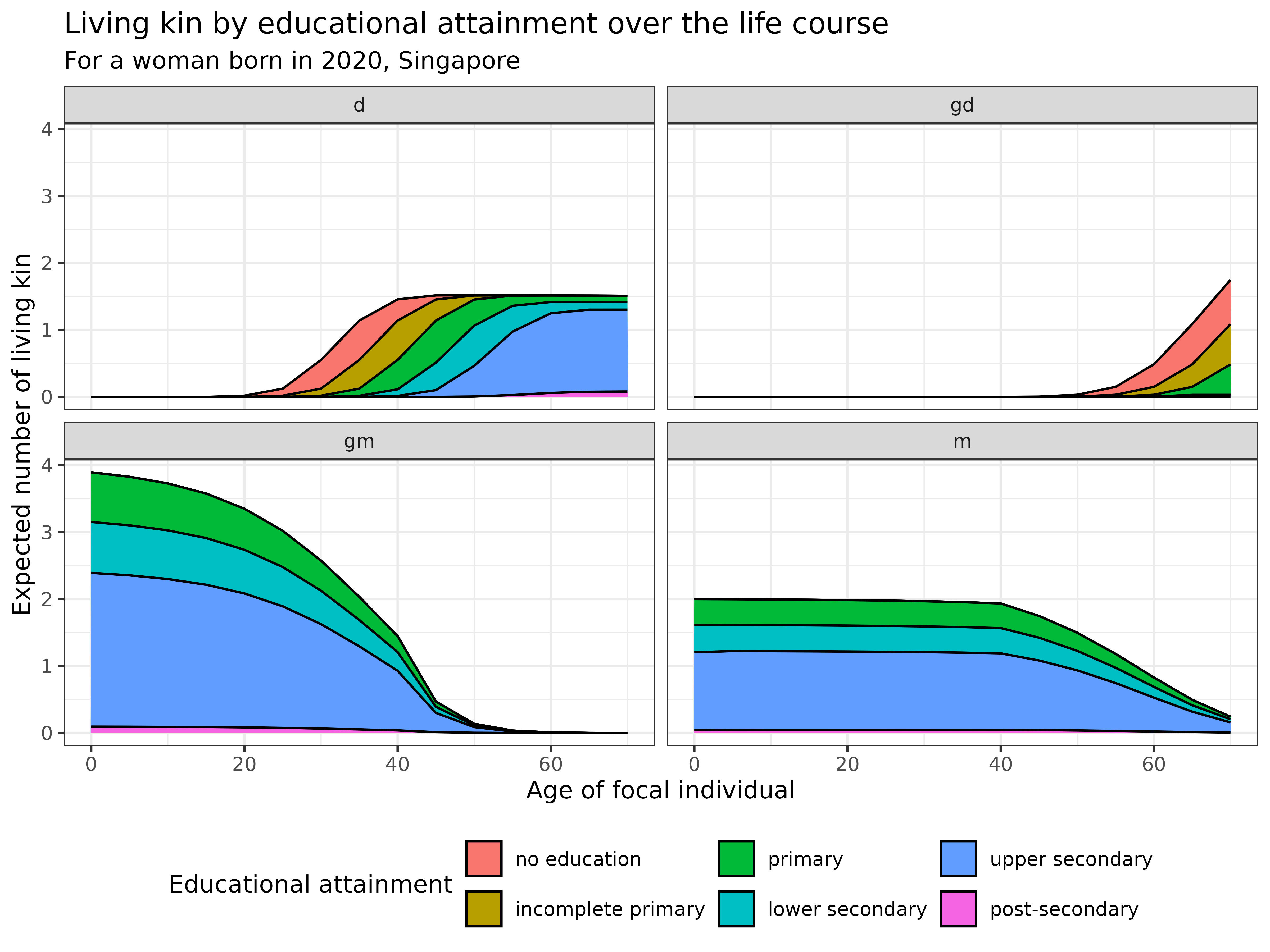
Interpretation This visualization captures how educational expansion transforms family networks, showing the increasing educational diversity across generations in Singapore:
- The total number of living relatives peaks around age 40-50
- Relatives with upper secondary education (blue) constitute the largest proportion of the kinship network
- The educational composition of relatives changes dynamically across the life course
- At younger ages, relatives have lower educational attainment. As Focal ages, the proportion of higher-educated relatives (green, yellow, and red categories) increases
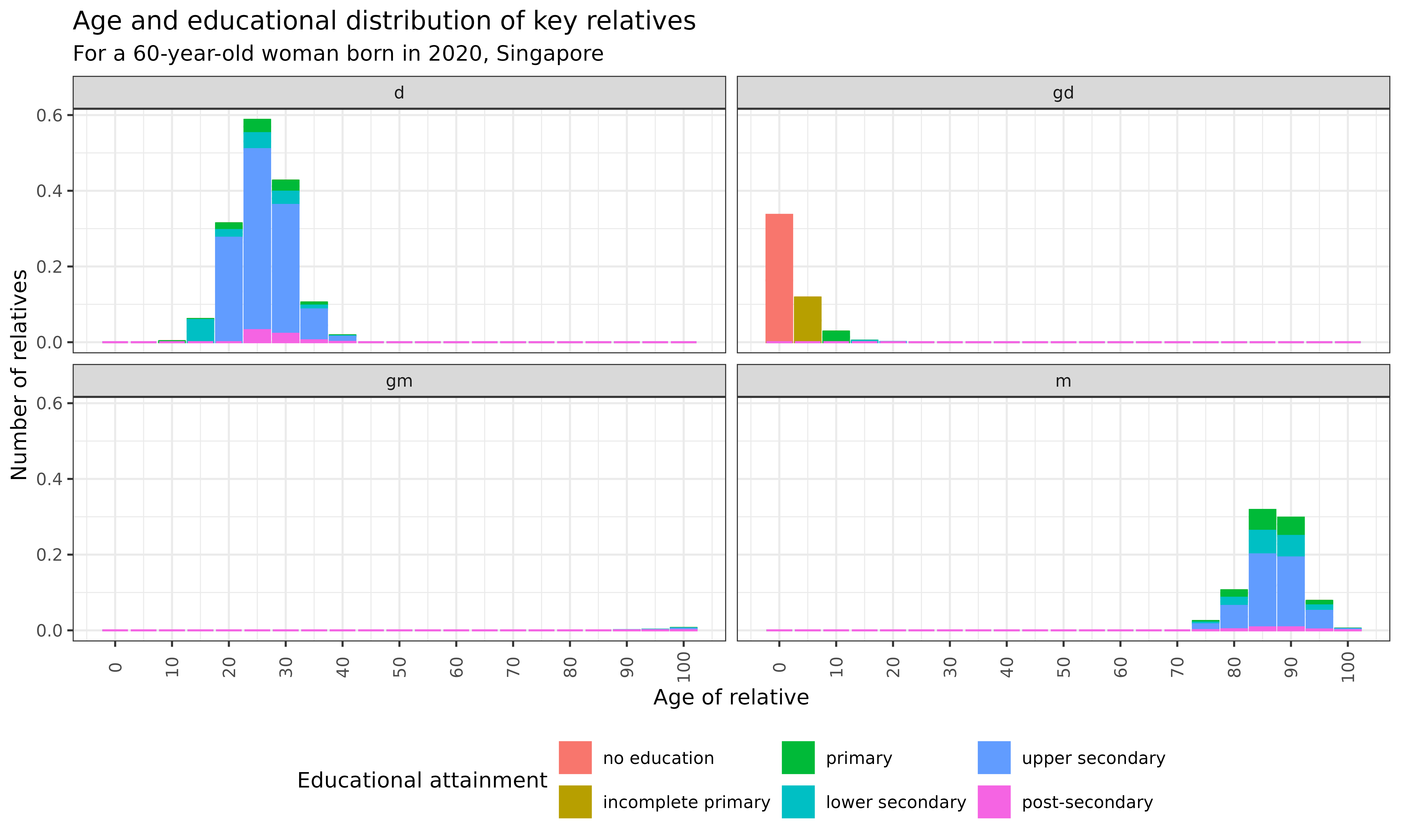
Let’s examine the age and educational distribution of key relatives when the focal individual is 60 years old:
kin_out_2020_2090$kin_full %>%
  filter(
    kin %in%  c("d", "gd", "m", "gm"),
    age_focal == 60,
    cohort == 2020
  ) %>%
  # rename_kin("2sex") %>%
  ggplot(aes(x = age_kin, y = living, color = stage_kin, fill = stage_kin)) +
  geom_bar(position = "stack", stat = "identity") +
  scale_x_continuous(breaks = c(0,10,20,30,40,50,60,70,80,90,100)) +
  labs(
    title = "Age and educational distribution of key relatives",
    subtitle = "For a 60-year-old woman born in 2020, Singapore",
    x = "Age of relative",
    y = "Number of relatives",
    fill = "Educational attainment",
    color = "Educational attainment"
  ) +
  facet_wrap(. ~ kin) +
  theme_bw() +
  theme(
    axis.text.x = element_text(angle = 90, vjust = 0.5),
    legend.position = "bottom"
  )
Interpretation: This visualization reveals the evolving educational composition of different types of relatives across the life course for a woman born in 2020 in Singapore:
- Children (d): Educational attainment increases with Focal’s age, showing a shift towards higher education levels
- Grandchildren (gd): Emerge later in life with a more diverse educational profile
- Grandparents (gm): Predominantly have upper secondary (blue) and lower secondary (teal) education
- Parents (m): Similar to grandparents, with a concentration of upper secondary education
Period Analysis of Kin by Education
Now let’s examine how the educational composition of specific relatives changes over time. First, let’s look at the educational attainment of descendants (children and grandchildren) of 60-year-old women across different calendar years:
kin_out_2020_2090$kin_summary %>%
  filter(
    kin %in% c("d", "gd"),
    age_focal == 60
  ) %>%
  # rename_kin(sex = "2sex") %>%
  summarise(count = sum(living), .by = c(stage_kin, kin, year)) %>%
  ggplot(aes(x = year, y = count, fill = stage_kin)) +
  geom_area(colour = "black") +
  labs(
    title = "Educational attainment of descendants over time",
    subtitle = "For women aged 60, Singapore, 2020-2090",
    y = "Expected number of descendants",
    x = "Year",
    fill = "Educational attainment"
  ) +
  facet_grid(. ~ kin) +
  theme_bw() +
  theme(legend.position = "bottom")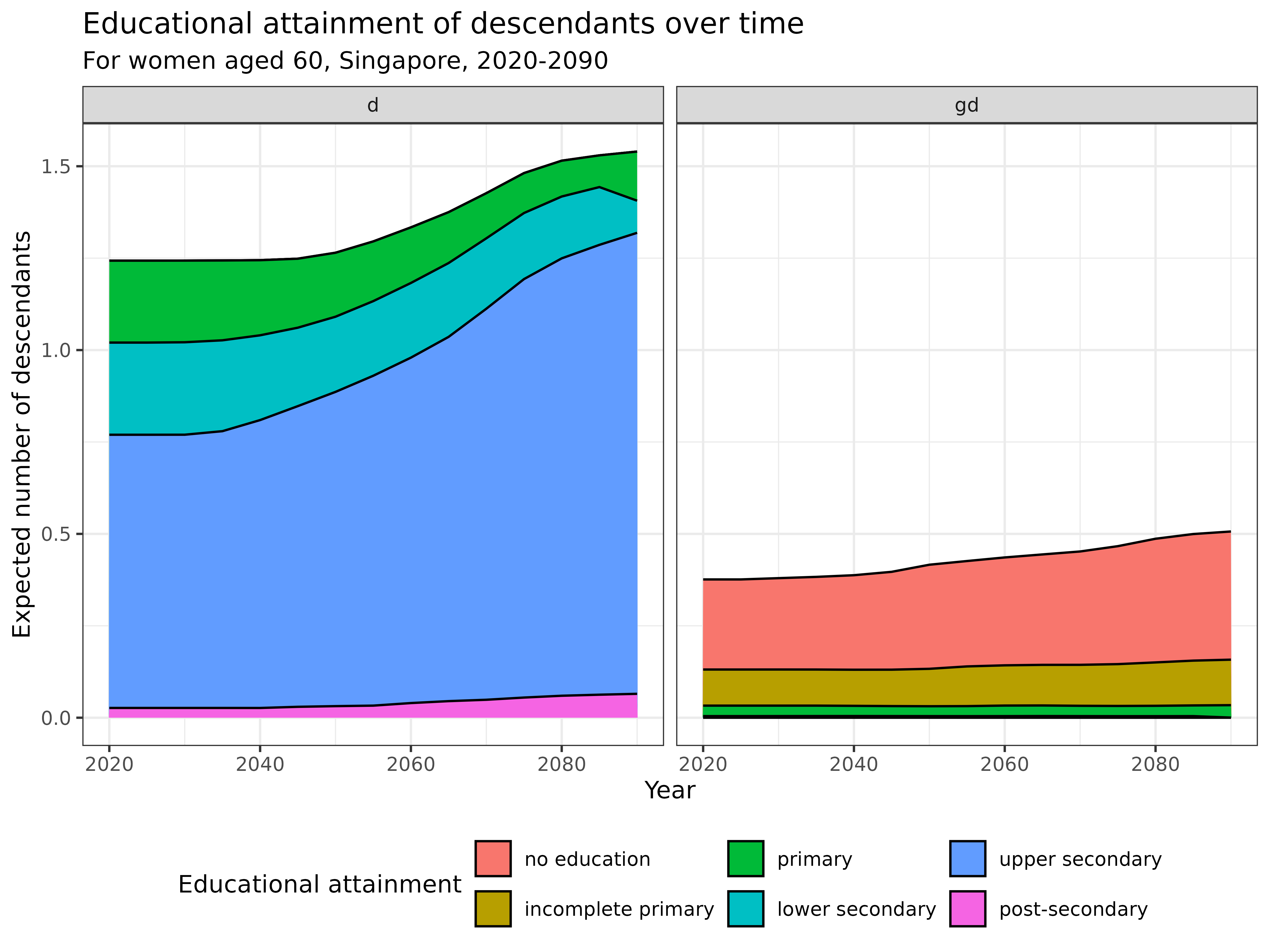
Interpretation:
- Children (d): Concentrated between ages 30-50, with upper secondary education (blue) being most prevalent
- Grandchildren (gd): Mostly young (under 20), with emerging educational diversity
- Grandparents (gm): No longer living at this point
- Parents (m): Clustered around ages 80-90, with upper secondary and lower secondary education dominating
Limitations and Assumptions
When implementing these models, we’ve made several simplifying assumptions due to data limitations:
For the UK parity model:
- Fertility rates vary with time and parity but are the same across sexes
- Mortality rates vary with time and sex but are the same across parity classes
- Parity progression probabilities vary with time but are the same across sexes
For the Singapore education model:
- Fertility rates vary over time and by education but are identical for both sexes
- Age-specific education transition probabilities vary over time but not by sex
- Educational transitions for young children follow Singapore’s Compulsory Education Act
- Demographic rates before 2020 are assumed stable (time-invariant)
These assumptions should be kept in mind when interpreting the results.
Conclusion
In this vignette, we’ve implemented two-sex time-varying multi-state kinship models—the most comprehensive demographic kinship framework currently available. By integrating age, sex, time, and stage dimensions, these models provide unprecedented insights into family structures and their evolution.
Our two examples demonstrated the analytical power of this integrated approach:
- The parity example revealed how reproductive patterns shape family structures differently for males and females across historical periods
- The education example showed how educational expansion transforms kinship networks, creating increasingly educated family systems over time
These comprehensive models have numerous applications across disciplines:
- Understanding intergenerational transmission of socioeconomic status
- Analyzing care needs and support networks in diverse populations
- Projecting how family structures might evolve under different demographic scenarios
- Exploring how education, health, marriage, and other characteristics intersect with kinship